Using TFReocrd File

Using TFReocrd File

• 이전 Post에서 TFRecord File Format을 만드는 방법에 대해서 알아보았습니다.

• 이번 Post에서는 지난 번에 작성한 TFRecord Dataset으로 Image Classification을 해보겠습니다.

• TFRecord는 Tensorflow와 함께 사용할 때 최고의 성능을 보여줍니다. 그래서, 가능하면 모든 Code들은 Tensorflow에서 제공하는 Function들을 사용해서 작성해 보도록 하겠습니다.

0. Prepare

• 필요한 Module을 Load합니다.

import tensorflow as tf
from tqdm import tqdm
from sklearn.model_selection import train_test_split

• Batch Size와 Prefetch할 Size를 미리 정의합니다.

class CFG:
    BATCH_SIZE = 32
    BUFFER_SIZE = 500

• 추후에 map에 적용하기 위해서 TFRecord File들의 Full Path를 구해놓습니다.

Cat_Fearue_File_List = tf.io.gfile.listdir("./PetImages/Cat/TFRecord")
Cat_Fearue_File_List = list(map(lambda x:"./PetImages/Cat/TFRecord/" + x, Cat_Fearue_File_List))

print(len(Cat_Fearue_File_List))
Cat_Fearue_File_List[:10]

12427

['./PetImages/Cat/TFRecord/0.tfrecord',
 './PetImages/Cat/TFRecord/1.tfrecord',
 './PetImages/Cat/TFRecord/10.tfrecord',
 './PetImages/Cat/TFRecord/100.tfrecord',
 './PetImages/Cat/TFRecord/1000.tfrecord',
 './PetImages/Cat/TFRecord/10000.tfrecord',
 './PetImages/Cat/TFRecord/10001.tfrecord',
 './PetImages/Cat/TFRecord/10002.tfrecord',
 './PetImages/Cat/TFRecord/10003.tfrecord',
 './PetImages/Cat/TFRecord/10004.tfrecord']

Dog_Fearue_File_List = tf.io.gfile.listdir("./PetImages/Dog/TFRecord")
Dog_Fearue_File_List = list(map(lambda x:"./PetImages/Dog/TFRecord/" + x, Dog_Fearue_File_List))

print(len(Dog_Fearue_File_List))
Dog_Fearue_File_List[:10]

12397

['./PetImages/Dog/TFRecord/0.tfrecord',
 './PetImages/Dog/TFRecord/1.tfrecord',
 './PetImages/Dog/TFRecord/10.tfrecord',
 './PetImages/Dog/TFRecord/100.tfrecord',
 './PetImages/Dog/TFRecord/1000.tfrecord',
 './PetImages/Dog/TFRecord/10000.tfrecord',
 './PetImages/Dog/TFRecord/10001.tfrecord',
 './PetImages/Dog/TFRecord/10002.tfrecord',
 './PetImages/Dog/TFRecord/10003.tfrecord',
 './PetImages/Dog/TFRecord/10004.tfrecord']

1. Train & Validation Set Split

• Train시에 사용할 Train / Val. Set을 분리하겠습니다.

• Cat / Dog 별로 동일한 8:2로 나누겠습니다.

Cat_Train_File_List, Cat_Val_File_List = train_test_split(Cat_Fearue_File_List, test_size=0.2, random_state=123)

print("Cat Train : ",len(Cat_Train_File_List) , "Cat Val. : ",len(Cat_Val_File_List))

Cat Train :  9941 Cat Val. :  2486

Dog_Train_File_List, Dog_Val_File_List = train_test_split(Dog_Fearue_File_List, test_size=0.2, random_state=123)

print("Dog Train : ",len(Dog_Train_File_List) , "Dog Val. : ",len(Dog_Val_File_List))

Dog Train :  9917 Dog Val. :  2480

• Cat / Dog의 Train File List와 Val. File List를 합칩니다.

Train_Feature_File_List = Cat_Train_File_List + Dog_Train_File_List

Val_Feature_File_List = Cat_Val_File_List + Dog_Val_File_List

print(len(Train_Feature_File_List) , len(Val_Feature_File_List) )

19858 4966

• 잘 섞어줍니다.

Train_Feature_File_List = tf.random.shuffle(Train_Feature_File_List)

Train_Feature_File_List

<tf.Tensor: shape=(19858,), dtype=string, numpy=
array([b'./PetImages/Dog/TFRecord/10425.tfrecord',
       b'./PetImages/Cat/TFRecord/3119.tfrecord',
       b'./PetImages/Cat/TFRecord/5364.tfrecord', ...,
       b'./PetImages/Dog/TFRecord/9267.tfrecord',
       b'./PetImages/Dog/TFRecord/12042.tfrecord',
       b'./PetImages/Dog/TFRecord/551.tfrecord'], dtype=object)>

Val_Feature_File_List = tf.random.shuffle(Val_Feature_File_List)

Val_Feature_File_List

<tf.Tensor: shape=(4966,), dtype=string, numpy=
array([b'./PetImages/Dog/TFRecord/4587.tfrecord',
       b'./PetImages/Cat/TFRecord/387.tfrecord',
       b'./PetImages/Cat/TFRecord/5345.tfrecord', ...,
       b'./PetImages/Dog/TFRecord/2247.tfrecord',
       b'./PetImages/Dog/TFRecord/12447.tfrecord',
       b'./PetImages/Cat/TFRecord/9419.tfrecord'], dtype=object)>

2. Making Dataset

• 이제 TFRecord File을 읽어서 Dataset을 만들도록 하겠습니다.

• 전체적인 순서는
  • TFRecord File들의 Full Path를 가지고 Dataset 생성
  • TFRecord File을 읽어서 Contents를 읽어오는 Map Function 작성 / 적용
  • Dataset에 shuffle / batch / prefetch 적용
  • Train에 적용
• 하나씩 알아보겠습니다.

2.1. Map Function

• TFRecord File의 내용을 Decoding하는 Function입니다.

• def map_fn(serialized_example):
  • Parameter로 넘어오는 serialized_example는 TFRecord File의 Full Path입니다.
  • 아래쪽에 TFRecordDataset을 이용해서 Dataset을 만들때 Parameter로 사용하는 값이 serialized_example로 넘어오는 것입니다.

• feature = { ‘Feature’: tf.io.FixedLenFeature([49*1280], tf.float32), ‘Label’: tf.io.FixedLenFeature([1], tf.int64) }

  • 우리가 읽을 TFRecord File의 구조를 정의하는 부분입니다.
  • ‘Feature’라는 Data는 Float형, 길이가 62720이며, ‘Label’이라는 Data는 Type이 Int형, 길이가 1이라는 뜻입니다.
  • 가만히 생각해 보면, 우리가 다른 사람이 작성한 TFRecord File을 읽어야 하는 경우에는 이러한 구조를 모르면 Decoding할 수가 없습니다.
  • 즉, TFRecord Format으로 Dataset을 배포할 때는 반드시 이런 구조 정보를 함께 알려주어야 하는 것입니다.

• example = tf.io.parse_single_example(serialized_example, feature)
  • 실제 File을 읽어서 위에서 정의한 구조대로 Decoding하는 부분입니다.

• example[‘Feature’] = tf.reshape( example[‘Feature’] , (7,7,1280) )
  • 우리가 TFRecord File을 저장할 때, Shape을 Flatten했기 때문에, 원래 모양대로 원상 복구합니다.

• tf.squeeze( tf.one_hot(example[‘Label’] , depth=2) )
  • Label은 Cat인 경우 0, Dog인 경우에 1입니다.
  • One Hot 형식으로 변경하는 부분입니다.

def map_fn(serialized_example):

    feature = {
        'Feature': tf.io.FixedLenFeature([49*1280], tf.float32),
        'Label': tf.io.FixedLenFeature([1], tf.int64)
    }
    
    example = tf.io.parse_single_example(serialized_example, feature)
    
    example['Feature'] = tf.reshape( example['Feature'] , (7,7,1280) )
    
    return example['Feature'], tf.squeeze( tf.one_hot(example['Label'] , depth=2) )

2.2. Define Dataset

• 우리는 TFRecord File List가 있기 때문에, Dataset 생성에 tf.data.TFRecordDataset을 사용하도록 하겠습니다.

Train_Dataset = tf.data.TFRecordDataset( Train_Feature_File_List )
Val_Dataset = tf.data.TFRecordDataset( Val_Feature_File_List )

Train_Dataset

<TFRecordDatasetV2 shapes: (), types: tf.string>

Val_Dataset

<TFRecordDatasetV2 shapes: (), types: tf.string>

• Dataset도 만들었고, Dataset에 적용할 Map Function도 만들었으니 이제 shuffle / batch / prefetch를 적용합니다.

Train_Dataset = Train_Dataset.map(map_fn , 
                      num_parallel_calls=tf.data.experimental.AUTOTUNE)

Train_Dataset = Train_Dataset.shuffle(CFG.BUFFER_SIZE).batch(CFG.BATCH_SIZE)
Train_Dataset = Train_Dataset.prefetch(buffer_size=tf.data.experimental.AUTOTUNE)

Val_Dataset = Val_Dataset.map(map_fn , 
                      num_parallel_calls=tf.data.experimental.AUTOTUNE)

Val_Dataset = Val_Dataset.shuffle(CFG.BUFFER_SIZE).batch(CFG.BATCH_SIZE)
Val_Dataset = Val_Dataset.prefetch(buffer_size=tf.data.experimental.AUTOTUNE)

• 제대로 읽는지 하나만 살펴볼까요?

for batch in Train_Dataset.take(1):
    batch

print(batch)
batch[1].numpy()

(<tf.Tensor: shape=(32, 7, 7, 1280), dtype=float32, numpy=
array([[[[-1.30283579e-01, -1.79280803e-01, -2.73918390e-01, ...,
          -2.35235289e-01, -2.51564652e-01, -1.24651089e-01],
         [-2.23974511e-01, -2.69972891e-01, -2.78214544e-01, ...,
          -1.61265686e-01, -2.63588488e-01,  4.82403219e-01],
         [-9.15986970e-02, -7.91421384e-02, -2.09058121e-01, ...,
          -2.46901169e-01, -2.35181734e-01, -2.75620580e-01],
         ...,
         [-4.28934097e-02, -3.80189456e-02, -9.37430859e-02, ...,
          -2.70000398e-01, -2.56699502e-01,  3.71812642e-01],
         [-3.37041589e-03,  2.37213349e+00, -2.73799729e-02, ...,
          -2.78330237e-01, -2.63371170e-01, -2.72408187e-01],
         [-2.69764900e-01, -9.48898420e-02, -6.93319291e-02, ...,
          -2.59258837e-01, -2.78016418e-01, -2.23277569e-01]],

        [[-2.40731761e-01, -1.49252594e-01, -1.29014462e-01, ...,
          -3.48842107e-02, -2.78116941e-01,  1.21828353e+00],
         [-2.78438926e-01,  5.36722839e-01, -1.36655658e-01, ...,
          -6.23840746e-03, -2.26522133e-01,  1.85954738e+00],
         [-6.25507459e-02, -1.00828111e-01, -1.55045748e-01, ...,
          -4.72838171e-02, -1.98967606e-01, -2.27459908e-01],
         ...,
         [-4.31086839e-04,  2.16324544e+00, -1.06345741e-02, ...,
          -3.63434367e-02, -3.13317887e-02,  9.24772203e-01],
         [-1.53233509e-06,  1.35951967e+01, -7.76352419e-04, ...,
          -4.41170437e-03, -2.31151477e-01, -2.63853192e-01],
         [-6.46062661e-03,  4.92377949e+00, -1.39266048e-02, ...,
          -5.87231778e-02,  1.09022892e+00, -2.71575540e-01]],

        [[-1.42593503e-01,  3.51380378e-01, -2.29087830e-01, ...,
          -9.77664907e-03, -2.43833497e-01,  6.59770250e-01],
         [-6.03562184e-02,  2.67279983e+00, -8.22568163e-02, ...,
          -3.87481693e-03, -3.45014818e-02,  2.45907426e+00],
         [-6.38377480e-03,  4.15273046e+00, -1.50325801e-02, ...,
          -8.94669294e-02, -1.27345668e-02, -2.78422236e-01],
         ...,
         [-3.85519373e-03, -1.10767812e-01, -3.39450780e-03, ...,
          -1.03545524e-02, -8.26057419e-03,  1.70724523e+00],
         [-5.78504521e-04,  6.60518837e+00, -2.84841983e-04, ...,
          -3.46982223e-03, -2.71046907e-02, -9.67810899e-02],
         [-5.40567897e-02, -2.77622372e-01, -3.78229097e-02, ...,
          -6.76211938e-02, -2.77685404e-01, -2.49596104e-01]],

        ...,


        [[ 2.25460219e+00, -2.29545057e-01,  7.19489276e-01, ...,
          -1.46996761e-02, -2.56974429e-01,  2.10201070e-01],
         [ 9.66896489e-02, -2.15796664e-01, -2.50947535e-01, ...,
          -2.59889185e-01, -2.60895252e-01,  1.05790734e-01],
         [-2.78464437e-01, -2.75186807e-01, -2.66715109e-01, ...,
          -2.64783144e-01, -1.05178565e-01,  4.61720973e-01],
         ...,
         [ 1.15485799e+00, -1.55356184e-01, -1.62961870e-01, ...,
          -7.94149265e-02, -2.78311014e-01,  7.28313923e-01],
         [ 2.17598176e+00, -8.69607255e-02,  2.29728460e-01, ...,
          -1.48992896e-01,  2.41546303e-01,  4.84176666e-01],
         [ 1.63772357e+00, -4.06442173e-02,  1.13258696e+00, ...,
          -2.36238405e-01, -2.71336257e-01,  6.56960234e-02]]]],
      dtype=float32)>, <tf.Tensor: shape=(32, 2), dtype=float32, numpy=
array([[0., 1.],
       [0., 1.],
       [1., 0.],
       [1., 0.],
       [1., 0.],
       [0., 1.],
       [0., 1.],
       [0., 1.],
       [0., 1.],
       [0., 1.],
       [1., 0.],
       [0., 1.],
       [0., 1.],
       [1., 0.],
       [0., 1.],
       [1., 0.],
       [1., 0.],
       [1., 0.],
       [0., 1.],
       [1., 0.],
       [0., 1.],
       [0., 1.],
       [1., 0.],
       [0., 1.],
       [1., 0.],
       [1., 0.],
       [0., 1.],
       [1., 0.],
       [1., 0.],
       [1., 0.],
       [1., 0.],
       [1., 0.]], dtype=float32)>)





array([[0., 1.],
       [0., 1.],
       [1., 0.],
       [1., 0.],
       [1., 0.],
       [0., 1.],
       [0., 1.],
       [0., 1.],
       [0., 1.],
       [0., 1.],
       [1., 0.],
       [0., 1.],
       [0., 1.],
       [1., 0.],
       [0., 1.],
       [1., 0.],
       [1., 0.],
       [1., 0.],
       [0., 1.],
       [1., 0.],
       [0., 1.],
       [0., 1.],
       [1., 0.],
       [0., 1.],
       [1., 0.],
       [1., 0.],
       [0., 1.],
       [1., 0.],
       [1., 0.],
       [1., 0.],
       [1., 0.],
       [1., 0.]], dtype=float32)

• take(1)만 해도, Batch Size만큼 읽는다는 것을 알 수 있습니다.

• 내용을 보니 제대로 읽어오는 것 같습니다.

3. Model Define

• Data도 준비되었으니, EfficientNet에서 추출한 Feature를 분류할 Simple Dense Net을 하나 정의하겠습니다.

• Input Shape 신경 써주고, 적당하게 만들어 줍니다.

model = tf.keras.Sequential()

model.add( tf.keras.layers.InputLayer(input_shape=(7,7,1280)) )
model.add( tf.keras.layers.GlobalAveragePooling2D() )

model.add( tf.keras.layers.BatchNormalization() )
model.add( tf.keras.layers.Dropout(0.25) )
model.add( tf.keras.layers.Dense(256 , activation='relu') )

model.add( tf.keras.layers.BatchNormalization() )
model.add( tf.keras.layers.Dropout(0.25) )
model.add( tf.keras.layers.Dense(64 , activation='relu') )

model.add( tf.keras.layers.BatchNormalization() )
model.add( tf.keras.layers.Dropout(0.25) )
model.add( tf.keras.layers.Dense(2 , activation='softmax') )

model.summary()

Model: "sequential"
_________________________________________________________________
Layer (type)                 Output Shape              Param #   
=================================================================
global_average_pooling2d (Gl (None, 1280)              0         
_________________________________________________________________
batch_normalization (BatchNo (None, 1280)              5120      
_________________________________________________________________
dropout (Dropout)            (None, 1280)              0         
_________________________________________________________________
dense (Dense)                (None, 256)               327936    
_________________________________________________________________
batch_normalization_1 (Batch (None, 256)               1024      
_________________________________________________________________
dropout_1 (Dropout)          (None, 256)               0         
_________________________________________________________________
dense_1 (Dense)              (None, 64)                16448     
_________________________________________________________________
batch_normalization_2 (Batch (None, 64)                256       
_________________________________________________________________
dropout_2 (Dropout)          (None, 64)                0         
_________________________________________________________________
dense_2 (Dense)              (None, 2)                 130       
=================================================================
Total params: 350,914
Trainable params: 347,714
Non-trainable params: 3,200
_________________________________________________________________

• Optimizer 선택해서 설정하고, Compile한 후에 Train시작하겠습니다.

optimizer = tf.keras.optimizers.Adam(learning_rate=1e-2)

model.compile(optimizer=optimizer, 
              loss="categorical_crossentropy", metrics=["accuracy"]
             )

EPOCHS = 5

hist = model.fit(Train_Dataset, 
                 epochs=EPOCHS, 
                 validation_data=Val_Dataset, 
                 verbose=1)

Epoch 1/5
621/621 [==============================] - 285s 458ms/step - loss: 0.0579 - accuracy: 0.9812 - val_loss: 0.0319 - val_accuracy: 0.9887
Epoch 2/5
621/621 [==============================] - 362s 582ms/step - loss: 0.0383 - accuracy: 0.9867 - val_loss: 0.0371 - val_accuracy: 0.9881
Epoch 3/5
621/621 [==============================] - 384s 618ms/step - loss: 0.0339 - accuracy: 0.9892 - val_loss: 0.0327 - val_accuracy: 0.9895
Epoch 4/5
621/621 [==============================] - 473s 761ms/step - loss: 0.0355 - accuracy: 0.9880 - val_loss: 0.0291 - val_accuracy: 0.9899
Epoch 5/5
621/621 [==============================] - 436s 702ms/step - loss: 0.0331 - accuracy: 0.9902 - val_loss: 0.0357 - val_accuracy: 0.9895

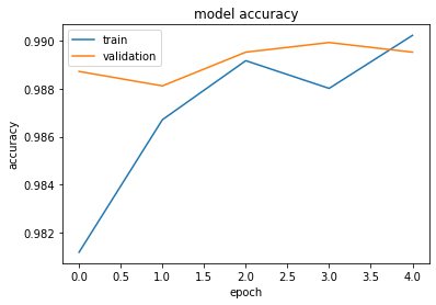
• 첫번째 Epoch에서 Train / Val. Set 모두에서 이미 높은 Accuracy를 보이네요.

• 제대로 동작하는 것 같네요.

import matplotlib.pyplot as plt

plt.plot(hist.history["accuracy"])
plt.plot(hist.history["val_accuracy"])
plt.title("model accuracy")
plt.ylabel("accuracy")
plt.xlabel("epoch")
plt.legend(["train", "validation"], loc="upper left")
plt.show()

4. Summary

• 이번 Post에서는 TFReocrd File Format을 읽어서 실제 Train에 적용시키는 방법까지 알아보았습니다.

• 중요한 것은 TFReocrd File을 사용하기 위해서는 해당 Dataset을 만들때 사용한 구조( Feature )를 반드시 알고 있어야 한다는 것입니다.