GAN (EN)
GAN(Generative Adversarial Nets)
0. Introduction
-
In 2014, Ian J. Goodfellow published a new model called Generative Adversarial Nets (GANs).
-
You read the paper by below link.
-
You would be easily aware that ‘Nets’ is well-known ‘Network’ but the exact meaning of ‘Adversarial’ or ‘Generative’ is a little bit difficult.
-
We will review what ‘GAN’ is in this post.
1. Background
1.1. Generative Model
-
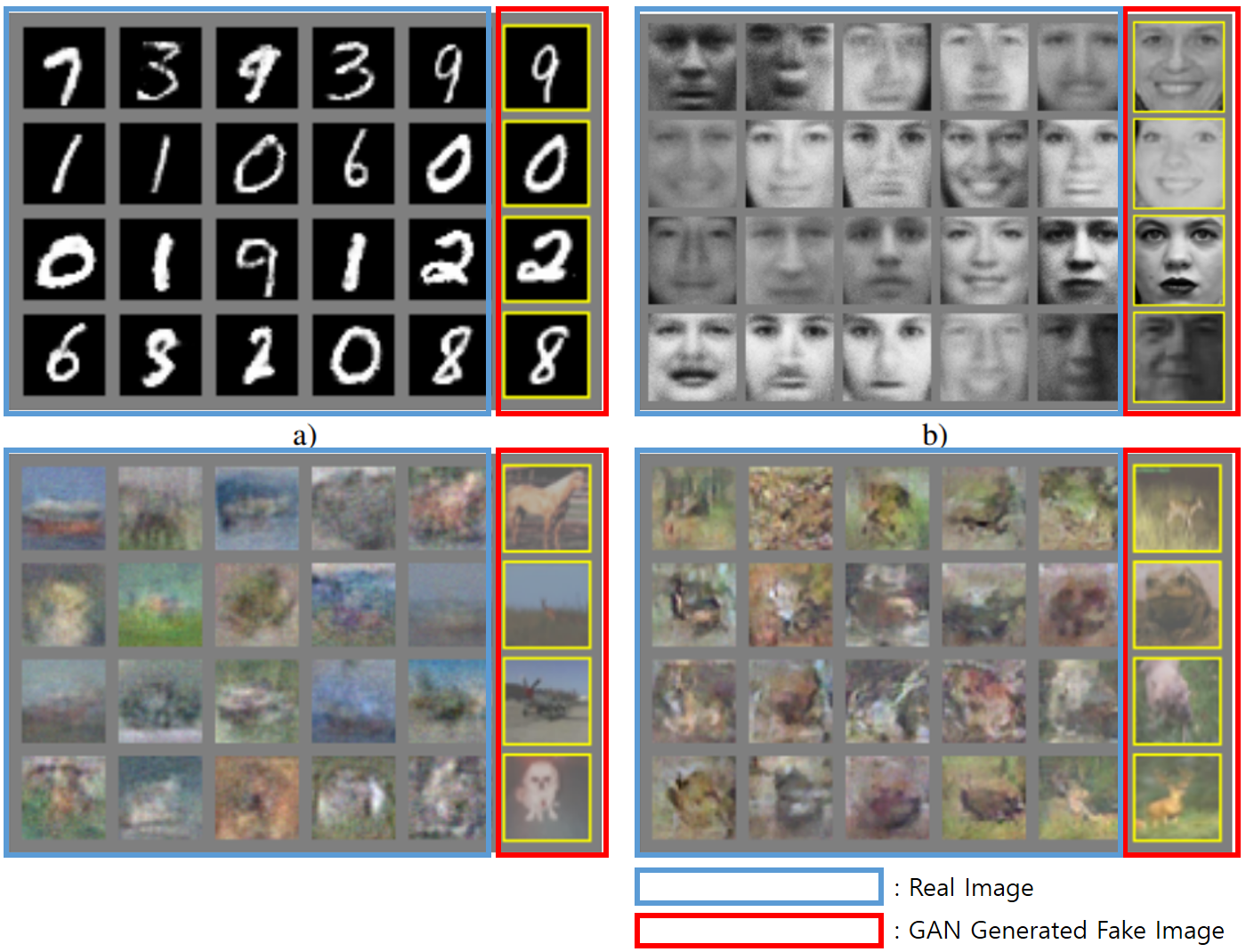
GAN is able to generate a data that is likely to exist but actually not exist.
-
Below image is from the paper of Ian Goodfellow.
-
The blue ones are real image and the red ones are generated by GAN. They seem to be real one.
1.2. Probability Distribution
- I really hate math., but we need to know the basic background of math.(Especially, probability) because the paper is full of math.
- First, let’s dive into ‘Probability Distribution’
-
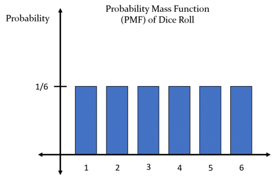
Probability Distribution is a function that represents the probability that a random variable has a certain value.
If a random variable X is the number of possible outcomes when a dice is rolled, P(X=1) is 1/6, and all P(X=1~6) have the same value (1/6).
- There are 2 kind of random distributions, Discrete Probability Distribution & Continuous Probability Distribution.
1.2.1. Discrete Probability Distribution
- Discrete probability distribution is a case in which the number of random variables X can be counted.
- The dice example at the previous example belongs to the discrete probability distribution.
1.2.2. Continuous Probability Distribution
- Continuous Probability Distribution is a probability distribution when the number of random variables X cannot be accurately counted.
- Since the number of random variables X cannot be counted accurately, in this case, the probability distribution is expressed using the probability density function.
- Examples of this might be things like height or running performance.
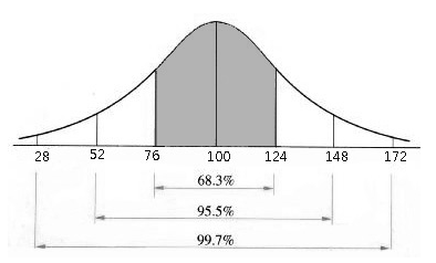
- Normal distribution can also be called continuous probability distribution.
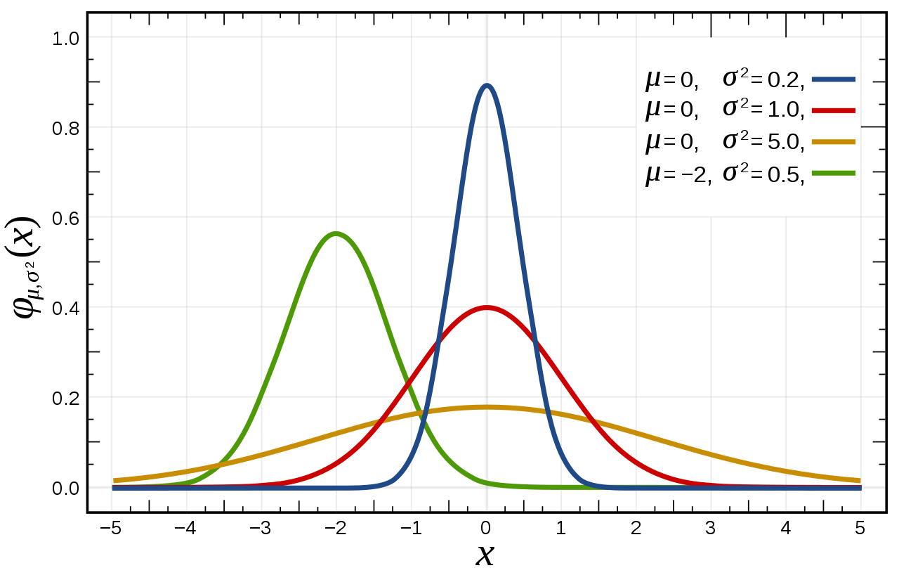
- In reality, the distribution of many data can be approximated as a normal distribution, and this fact is very useful for expressing and utilizing actual data.
- One of the example of a normal distribution in the real world is IQ.
1.2.3. Probability Distribution of Image
- The term ‘Probability Distribution for an Image’ may seem a bit cryptic.
- If you think about it, an image can also be expressed as a point in a multidimensional feature space. ( High-dimensional Vector or Matrix )
- In other words, a model that approximates this probability distribution by expressing the image data as a probability distribution can be learned using GAN.
- ‘What probability distribution is there in image data?’
- Human faces have statistical averages.
- For example, there could be values such as the relative positions of the eyes, nose, mouth, etc.
- This means that these numbers can be expressed as probability distributions.
- In Image, various features can each be a random variable, which means a distribution.
- For example, below one represents ‘Multivariate Probability Distribution’.

2. Generative Model
2.1. Generative Model vs Discriminative Model
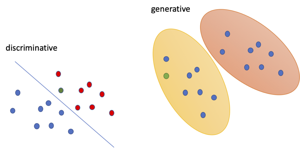
- Machine learning or deep learning models before GAN learn patterns from data, the model outputs a specific value based on the learning result for new data and discriminates it based on value from model output.
- In other words, a discriminative model is to learn a specific decision boundary.
- On the other hand, a generative model is a model that learns probability distribution from sample data and creates a probability distribution similar to the learned probability distribution although it does not actually exist.
- This means that generative models learn statistical means and generate similar probability distributions.
2.2. Purpose of Generative Model
- As mentioned before, the purpose of generative models is to generate a model G that approximates the probability distribution.
- The generative model is trained through the following process and learned to approximate the probability distribution of the original data.
- If G is well trained, it will be possible to easily generate data with similar statistical averages to the original data.
- A more detailed explanation of this graph will be given later.
3. GAN(Generative Adversarial Nets)
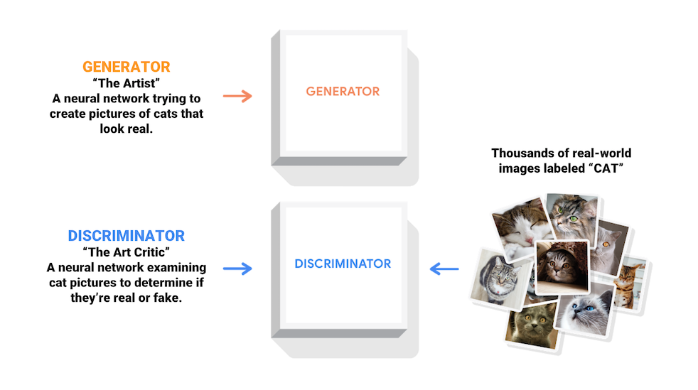
- GAN is a generative model using two networks, a generator and a discriminator.
- The figure below is taken from Tensorflow’s GAN page and shows the basic structure of GAN.
- There are two main models, a generator and a discriminator.
- Generator learns the original data probability distribution and is trained to generate data similar to the original probability distribution and the Discriminator learns to distinguish whether the data generated by the generator is real or fake.
- The ultimate purpose of these two models is to improve the performance of the generator by conducting competitive learning.
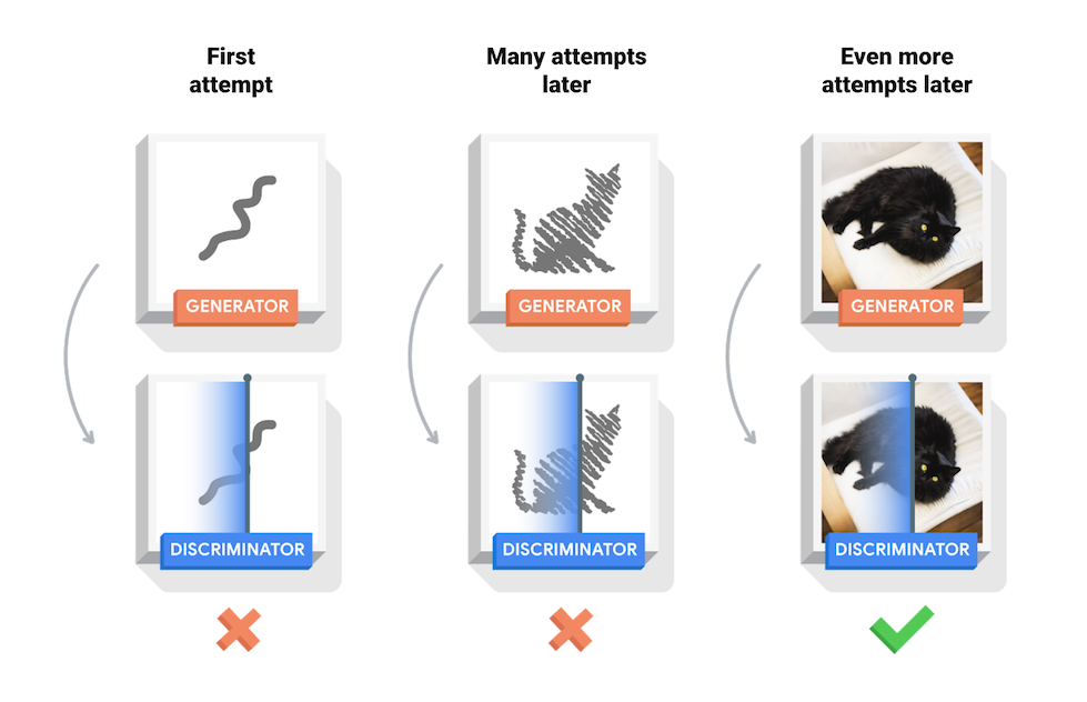
- During the training process, the generator will gradually become better at creating realistic images, and the discriminator will gradually become better at distinguishing between real and fake. This process reaches equilibrium when the discriminator can no longer distinguish the real image from the fake image generated by generator.
- The role of the discriminator is to help the generator G learn well, and the final goal to get is the generator (G).
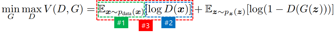
- The following formula is from Ian’s paper and explains the operation of GAN well.

- Let’s understand the meaning of the above formulas one by one.

- #1 : The whole function V consists of D and G.
- #2: D learns to the direction of maximizing the entire equation V.
- #3: Conversely, G learns to the direction of minimizing the entire equation V.
- First, let’s look at the terms containing D.
- #1 : Take one data(x) from the probability distribution P.
- #2: Taking the log of the result of putting the extracted data(x) into the function D,
- #3 : Calculate expected value(E). You may consider that expected value means the average value.
- Let’s look at terms that contain G.

- #1: Probability distribution z is a latent vector and can be also noise vector. Pick one z from the latent vector.
- #2 : Put z into G, and take the log after subtracting the result of putting the value generated by G into D from 1.
- #3 : Take the log and find the overall expected value (average).
- In the above formula, G(z) is a generator, which creates a new data instance from latent vector z.
- D(x) returns the probability that the probability distribution x is real or fake. ( Real : 1 , Fake : 0 )
- It can be seen that V is optimized by D and G and as a result, G can generate plausible data, according to paper.
3.1. Calculation of Expected Values
- E (expected value) is calculated in the above formula but the simplest way to implement it in the actual code is to simply obtain the values for all data and then find the average.
- Usually, E (expected value) is used when you want to find the average value when dealing with a lot of data.

- The above expression means to calculate the expected value of logD(x) by extracting x from the original data distribution.
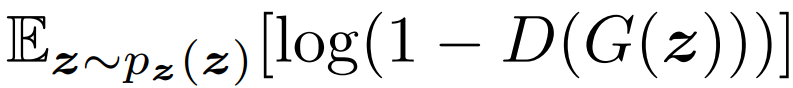
- The above formula means that the expected value of log(1 - D(G(z))) is calculated by taking z from the latent vector.
- In the actual code, you can calculate all data in a loop.
3.2. Train Process
- The goal of learning is described by the following formula.
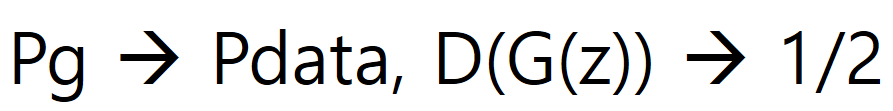
- When G is finished learning, D cannot distinguish the real / fake generated by G, so the probability is returned 1/2.
- Please refer to the proof of the above formula as it is a very complex formula in Paper.
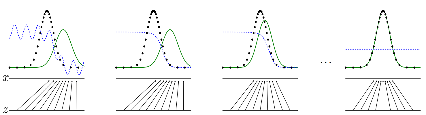
- Let’s look at the learning process again with the picture showed earlier.
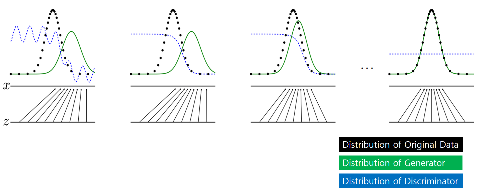
- The black probability distribution indicates the probability distribution of the original data, the green indicates the probability distribution generated by the generator, and the blue indicates the return value of the discriminator.
- As learning progresses from left to right, it indicates that the probability distribution generated by the generative model follows the original probability distribution, and the discriminator converges to 1/2.
3.3. Learning Algorithm of GAN
- The pseudo code below is the code shown in the paper.

- Train D (Discriminator) first.
- Extracts m samples from the latent vector and extracts m samples from the original data.
- D proceeds training to the direction of maximizing the equation while observing the gradient.
- Repeat training D k times in the same way as above.
- Next, train G (Generator). Extract m samples from the latent vector.
- Training proceeds to the direction of minimizing the formula value at the bottom.
- In this post, I briefly reviewed the GAN paper.
- In the next post, I will learn about GAN by running the actual code.