Tensorflow Input Pipeline(EN)
Tensorflow Input Pipeline
-
It is a very tedious and arduous process from the given data to the data format required for the train.
-
We should set the shape according to the input format of the model and consider data augmentation as well.
-
Most importantly, if there are tens or millions of data, performance is also an important consideration.
-
To solve all these concerns, Tensorflow has prepared tf.data and tf.data.Dataset module.
-
In this post, I would like to explain how to create an efficient data input pipeline using Tensorflow.
-
In tf.data.Dataset, the 4 fuctions, map / prefetch / cache / batch, are the most important and I will also check how to use them through an examples.
0. Example Dataset Download
-
There is a dataset which is often used when explaining the Tensorflow Input Pipeline.
- I will use using this dataset as well.
- You can download the dataset below link. Dataset Download
- After unzipping, the dataset is ready.
1. Exploring Dataset
import tensorflow as tf
import pandas as pd
import PIL
import PIL.Image
import pathlib
import matplotlib.pyplot as plt
import numpy as np
import os
-
Image files to be used for training are stored in a folder named ‘image’ and the label information for each image file is stored in ‘miml_labels_1.csv’ file.
-
First, let’s open and check the label information file.
df = pd.read_csv("./miml_dataset/miml_labels_1.csv")
df.head()
| Filenames | desert | mountains | sea | sunset | trees | |
|---|---|---|---|---|---|---|
| 0 | 1.jpg | 1 | 0 | 0 | 0 | 0 |
| 1 | 2.jpg | 1 | 0 | 0 | 0 | 0 |
| 2 | 3.jpg | 1 | 0 | 0 | 0 | 0 |
| 3 | 4.jpg | 1 | 1 | 0 | 0 | 0 |
| 4 | 5.jpg | 1 | 0 | 0 | 0 | 0 |
- ‘1’ is marked in the CSV file at the item corresponding to the object described in the file name and the image file.
- One thing that you should pay attention is that, in some cases, there might be multiple 1s for one image file.
LABELS=["desert", "mountains", "sea", "sunset", "trees"]
- Let’s check a file
data_dir = pathlib.Path("miml_dataset")
filenames = list(data_dir.glob('images/*.jpg'))
print("image count: ", len(filenames))
print("first image: ", str(filenames[0]) )
image count:  2000
first image:  miml_dataset\images\1.jpg
PIL.Image.open(str(filenames[0]))
- I make a string list that contains the full path of each image file to make Dataset easier.
fnames=[]
for fname in filenames:
    fnames.append(str(fname))

fnames[:5]
['miml_dataset\\images\\1.jpg',
 'miml_dataset\\images\\10.jpg',
 'miml_dataset\\images\\100.jpg',
 'miml_dataset\\images\\1000.jpg',
 'miml_dataset\\images\\1001.jpg']
2. Making Dataset
-
There are several ways to make Dataset, in this post, I’d like to choose tf.data.Dataset.from_tensor_slices() that is the most common and easy to use.
- In general, it’s used a file list as a parameter of from_tensor_slices() and preprocessd by .map() function, which is used a lot.
- It provides lots of flexibility.
- The total number of image file is 2000 and the list, fnames, has all the full path information of image files.
ds_size= len(fnames)
print("Number of images in folders: ", ds_size)
Number of images in folders: 2000
-
I pass ‘fnames’ to the parameter of from_tensor_slices()
-
Now, we have a Dataset
Note the fnames that go into the parameter of from_tensor_slices().
This is a list that stores the full path of image file
This is because it is closely related to the .map() function to be used later and the functions to be applied to .map().
filelist_ds = tf.data.Dataset.from_tensor_slices( fnames )
ds_size= filelist_ds.cardinality().numpy()
print("Number of selected samples for dataset: ", ds_size)
Number of selected samples for dataset: 2000
-
The total number of filelist_ds is 2000.
( cardinality() returns the total number of Dataset )
-
Let’s check whether Dataset we’ve created has correct data or not.
-
Let’s print out only 3 of them from the Dataset.
for a in filelist_ds.take(3):
    fname= a.numpy().decode("utf-8")
    print(fname)
    display(PIL.Image.open(fname))
miml_dataset\images\1.jpg

miml_dataset\images\10.jpg
miml_dataset\images\100.jpg
3. Making Label
-
Now that we have created a dataset to be used for train, let’s create a label according to it.
-
Label info. is in CSV file, right ?
df.head()
| Filenames | desert | mountains | sea | sunset | trees | |
|---|---|---|---|---|---|---|
| 0 | 1.jpg | 1 | 0 | 0 | 0 | 0 |
| 1 | 2.jpg | 1 | 0 | 0 | 0 | 0 |
| 2 | 3.jpg | 1 | 0 | 0 | 0 | 0 |
| 3 | 4.jpg | 1 | 1 | 0 | 0 | 0 |
| 4 | 5.jpg | 1 | 0 | 0 | 0 | 0 |
LABELS
['desert', 'mountains', 'sea', 'sunset', 'trees']
- 아래 Function은 Image File Full Path를 받아서 해당하는 Label 정보만을 Tensor형태로 return해 줍니다.
- The following function gets the image file full path and returns only the relevant label information in the form of Tensor.
def get_label(file_path):

    parts = tf.strings.split(file_path, '\\')

    file_name= parts[-1]

    # Dataframe에서 LABELS에 정의된 Column만 뽑아낸다.
    # .to_numpy()는 DataFrame인 Series를 ndarray 형태로 변환한다.
    #.squeeze()는 1차원인 축을 제거한다.
    labels= df[df["Filenames"]==file_name][LABELS].to_numpy().squeeze()

    return tf.convert_to_tensor(labels)
- Let’s check the function works correctly.
for a in filelist_ds.take(5):
    print("file_name: ", a.numpy().decode("utf-8"))
    print(get_label(a).numpy())
file_name:  miml_dataset\images\1.jpg
[1 0 0 0 0]
file_name:  miml_dataset\images\10.jpg
[1 1 0 0 0]
file_name:  miml_dataset\images\100.jpg
[1 0 0 1 0]
file_name:  miml_dataset\images\1000.jpg
[0 0 1 0 0]
file_name:  miml_dataset\images\1001.jpg
[0 0 1 0 0]
- OK. Good. I’ll use these values as label
4. Dataset Preprocessing
-
When data is put into the model for train, it must be converted into Tensor type.
-
The task we will do is image classification and through a series of processes, the data will need to be transformed to fit the shape required by model we have defined.
-
To do this, I make a function that read the image files, change the shape of data for the model and also create a label corresponding to it.
-
This operation will be applied to all the items of Dataset and will be used as a parameter of map() in the dataset.
-
The pre-train model to be used here is VGG16 and this model requires 32x32 input.
IMG_WIDTH, IMG_HEIGHT = 32 , 32
- The function below reads an image file and converts it into a float type Tensor. (It’s very convenient.)
def process_img(img):

    img = tf.image.decode_jpeg(img, channels=3)

    img = tf.image.convert_image_dtype(img, tf.float32)

    return tf.image.resize(img, [IMG_WIDTH, IMG_HEIGHT])
-
The following function generates and returns label information as well as image file.
-
Finally, I will apply ‘combine_images_labels()’ function to the .map() of Dataset.
- Please, take a look at the parameters & return value of the function.
-
I don’t know why Tensorflow made it so complicated, The parameter(file_path) of function to be applied to .map()(combine_images_labels()) is the value previously entered as the parameter of from_tensor_slices().
-
It means that we’ve made a Dataset by “filelist_ds = tf.data.Dataset.from_tensor_slices( fnames )” and fnames would be passed as file_path.
-
And the return values(‘img’ & ‘label’) will be the train & target values of .fit() function.
-
The doc. of Tensorflow would explain this complex relationship well, but actually not.
-
-
I think this is the most important part of writing Tensorflow Pipeline.
-
It is an important part of converting a given raw data file (Image, Sound, etc.) into a Tensor form that can be trained by model and I think that it is a part where individual capabilities and prowess can be well revealed.
-
If you use Tensorflow Function for all codes when writing this function, you can get much better performance.
- In the code below, you can see that the tf.io Module is used for the part that reads the image file. Moreover, as looking at process_img(), you can see that they all use tf. There is a reason. However, only one line in get_label() does not use the tf module. In this case, the usage of the .map() function is slightly different and we will also check it.
def combine_images_labels(file_path: tf.Tensor):

    img = tf.io.read_file(file_path)

    img = process_img(img)

    label = get_label(file_path)

    return img, label
- Dataset is divided into train & val set by 80:20
train_ratio = 0.80
ds_train=filelist_ds.take(ds_size*train_ratio)
ds_test=filelist_ds.skip(ds_size*train_ratio)

print("train size: ", ds_train.cardinality().numpy())
print("test size: ", ds_test.cardinality().numpy())
train size:  1600
test size:  400
-
Below code is an example to apply .map() function to Dataset.
-
tf.py_function is a part that defines a function to be applied to Dataset. Let’s apply the combine_images_labels()
-
If combine_images_labels() consists of pure Tensorflow module functions only, you can simply write the function name.
-
I’ll cover this next time
-
Setting num_parallel_calls to tf.data.experimental.AUTOTUNE. This part allows Tensorflow to dynamically allocate the pipeline as the background to improve performance.
-
Please be sure to apply prefetch().
ds_train = ds_train.map(lambda x:
                        tf.py_function(func=combine_images_labels,
                                       inp=[x],
                                       Tout=(tf.float32 , tf.int64)),
                        num_parallel_calls=tf.data.experimental.AUTOTUNE,
                        deterministic=False)

ds_train.prefetch(ds_size-ds_size*train_ratio)
<PrefetchDataset shapes: (<unknown>, <unknown>), types: (tf.float32, tf.int64)>
ds_test = ds_test.map(lambda x:
                      tf.py_function(func=combine_images_labels,
                                     inp=[x], Tout=(tf.float32,tf.int64)),
                      num_parallel_calls=tf.data.experimental.AUTOTUNE,
                      deterministic=False)

ds_test.prefetch(ds_size-ds_size*train_ratio)
<PrefetchDataset shapes: (<unknown>, <unknown>), types: (tf.float32, tf.int64)>
-
Let’s check the Dataset applied .map() work correctly.
-
Checking one train data from Dataset.
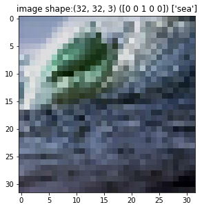
for image, label in ds_train.take(1):
    print("Image shape: ", image.shape)
    print("Label: ", label.numpy())
Image shape:  (32, 32, 3)
Label:  [1 0 0 0 0]
- Image shapes and labels to be used for training are all made correctly.
def covert_onehot_string_labels(label_string,label_onehot):
    labels=[]

    for i, label in  enumerate(label_string):
        if label_onehot[i]:
            labels.append(label)

    if len(labels)==0:
        labels.append("NONE")

    return labels
covert_onehot_string_labels(LABELS,[0,1,1,0,1])
['mountains', 'sea', 'trees']
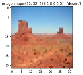
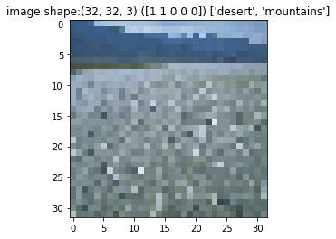
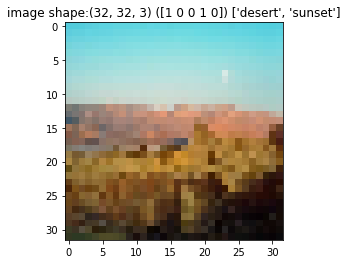
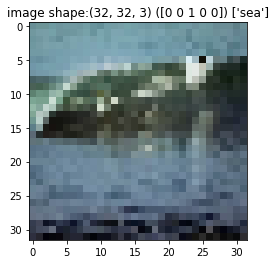
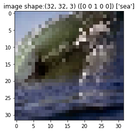
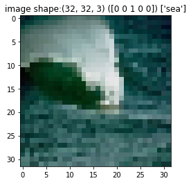
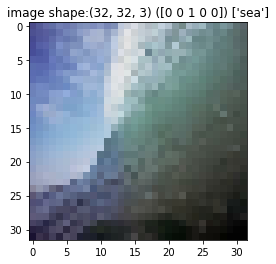
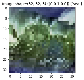
def show_samples(dataset):
    fig=plt.figure(figsize=(16, 16))
    columns = 3
    rows = 3

    print(columns*rows,"samples from the dataset")

    i=1
    for a,b in dataset.take(columns*rows):
        fig.add_subplot(rows, columns, i)
        plt.imshow(np.squeeze(a))
        plt.title("image shape:"+ str(a.shape)+" ("+str(b.numpy()) +") "+
                  str(covert_onehot_string_labels(LABELS,b.numpy())))
        i=i+1
        plt.show()
show_samples(ds_train)
9 samples from the dataset
print("Number of samples in train: ", ds_train.cardinality().numpy(),
      " in test: ",ds_test.cardinality().numpy())
Number of samples in train: 1600 in test: 400
5. Configure for Performance Enhancement
-
Now, it’s time to apply batch / cache / prefetch to boost up the performance
-
This is probably the reason to use Tensorflow Data Pipeline.
-
It is also available in official documents, so it would be nice to refer to it here.
- Reviewing at each item one by one,
- batch : Making one batch as much as the batch size from the dataset. It is the same as the conventional batch size concept.
- cache : The files corresponding to the dataset are cached in local storage or memory. Applying this behavior, you can see very fast performance from the next Epoch except for the first Epoch.
- prefetch : When prefetch is applied, it prepares for the next operation in advance during the train.
- Cache and prefetch have a very huge impact on performance improvement, so be sure to apply them.
BATCH_SIZE = 4
ds_train_batched = ds_train.batch(BATCH_SIZE).cache().prefetch(tf.data.experimental.AUTOTUNE)

ds_test_batched = ds_test.batch(BATCH_SIZE).cache().prefetch(tf.data.experimental.AUTOTUNE)
print("Number of batches in train: ", ds_train_batched.cardinality().numpy())
print("Number of batches in test: ", ds_test_batched.cardinality().numpy())
Number of batches in train:  400
Number of batches in test:  100
- As looking at the code above, you can see that batch / cache / prefetch were applied in order to both of Train / Val dataset.
6. Setup Model
-
Now, we’re prepared dataset for training.
-
Let’s use VGG16, which is simple to use.
-
Model definition and other configurations are general information, so we will not look at them in detail.
base_model = tf.keras.applications.VGG16(
    weights='imagenet',  # Load weights pre-trained on ImageNet.
    input_shape=(32, 32, 3), # VGG16 expects min 32 x 32
    include_top=False)  # Do not include the ImageNet classifier at the top.

base_model.trainable = False
number_of_classes = 5
inputs = tf.keras.Input(shape=(32, 32, 3))

x = base_model(inputs, training=False)
x = tf.keras.layers.GlobalAveragePooling2D()(x)
initializer = tf.keras.initializers.GlorotUniform(seed=42)

activation =  tf.keras.activations.softmax #None  # tf.keras.activations.sigmoid or softmax

outputs = tf.keras.layers.Dense(number_of_classes,
                             kernel_initializer=initializer,
                             activation=activation)(x)
model = tf.keras.Model(inputs, outputs)
model.compile(optimizer=tf.keras.optimizers.Adam(),
              loss=tf.keras.losses.CategoricalCrossentropy(), # default from_logits=False
              metrics=[tf.keras.metrics.CategoricalAccuracy()])
- Everything is ready.
model.fit(ds_train_batched,
          validation_data = ds_test_batched,
          epochs=10)
Epoch 1/10
400/400 [==============================] - 467s 1s/step - loss: 1.2755 - categorical_accuracy: 0.6988 - val_loss: 2.0400 - val_categorical_accuracy: 0.3975
Epoch 2/10
400/400 [==============================] - 6s 14ms/step - loss: 1.1283 - categorical_accuracy: 0.7206 - val_loss: 1.9769 - val_categorical_accuracy: 0.3975
Epoch 3/10
400/400 [==============================] - 6s 14ms/step - loss: 1.0616 - categorical_accuracy: 0.7394 - val_loss: 1.9540 - val_categorical_accuracy: 0.4175
Epoch 4/10
400/400 [==============================] - 6s 14ms/step - loss: 1.0220 - categorical_accuracy: 0.7538 - val_loss: 1.9391 - val_categorical_accuracy: 0.4275
Epoch 5/10
400/400 [==============================] - 5s 14ms/step - loss: 0.9927 - categorical_accuracy: 0.7606 - val_loss: 1.9297 - val_categorical_accuracy: 0.4400
Epoch 6/10
400/400 [==============================] - 5s 14ms/step - loss: 0.9689 - categorical_accuracy: 0.7669 - val_loss: 1.9246 - val_categorical_accuracy: 0.4525
Epoch 7/10
400/400 [==============================] - 5s 14ms/step - loss: 0.9487 - categorical_accuracy: 0.7738 - val_loss: 1.9227 - val_categorical_accuracy: 0.4550
Epoch 8/10
400/400 [==============================] - 5s 14ms/step - loss: 0.9311 - categorical_accuracy: 0.7744 - val_loss: 1.9233 - val_categorical_accuracy: 0.4625
Epoch 9/10
400/400 [==============================] - 6s 14ms/step - loss: 0.9155 - categorical_accuracy: 0.7775 - val_loss: 1.9257 - val_categorical_accuracy: 0.4625
Epoch 10/10
400/400 [==============================] - 6s 14ms/step - loss: 0.9015 - categorical_accuracy: 0.7806 - val_loss: 1.9296 - val_categorical_accuracy: 0.4650


<tensorflow.python.keras.callbacks.History at 0x20feaa60940>
-
Now, the train is over. To simply check the operation, I only rotated it 10 times.
-
The first epoch takes a lot of time to train, while the next epoch is very fast. That’s all thanks to cache / prefetch.
-
The acc. of the train set is low and the overfitting of the model is severe, but it is not important in this post, so I will skip it.
-
The key is to apply the following to the Dataset!