DCGAN Example (EN)
DCGAN Example
DCGAN Example
- In this post, I will take an example of DCGAN with code.
-
This example has been imported from below Tensorflow Tutorial Site.
- In this example, we will see that the trained model generates data similar to MNIST data after learning the probability distribution of MNIST dataset.
0. Import Package
- Load packages
- imageio is necessary when making GIF animation.
import glob
import imageio
import matplotlib.pyplot as plt
import numpy as np
import os
import PIL
from tensorflow.keras import layers
import time

from IPython import display
import tensorflow as tf
1. Loading Dataset & Preprocessing
- As mentioned earlier, Generator and Discriminator will train MNIST dataSet.
- After training, Generator will generate a letter similar to MNIST handwriting.
(train_images, train_labels), (_, _) = tf.keras.datasets.mnist.load_data()
Downloading data from https://storage.googleapis.com/tensorflow/tf-keras-datasets/mnist.npz
11493376/11490434 [==============================] - 11s 1us/step
train_images = train_images.reshape(train_images.shape[0], 28, 28, 1).astype('float32')
- Normalizing images to [-1, 1]
train_images = (train_images - 127.5) / 127.5
BUFFER_SIZE = 60000
BATCH_SIZE = 256
- Making dataset batch and shuffle.
train_dataset = tf.data.Dataset.from_tensor_slices(train_images).shuffle(BUFFER_SIZE).batch(BATCH_SIZE)
2. Making Model
- Implementing Generator & Discriminator by the way used in DCGAN paper.
2.1. Generator
- The generator accepts the noise(random) value as input to train to generate MNIST data.
- As you can see, it uses Tensorflow conv2dtranspose[TF.KERAS.LAYERS.CONV2DTRANSPOSE] (https://www.tensorflow.org/api_docs/python/tf/keras/layers/conv2dtranspose) for upsampling.
- Then, making Generator using Batch Normalization / ReLU / Tanh.
def make_generator_model():
    model = tf.keras.Sequential()
    model.add(layers.Dense(7*7*256, use_bias=False, input_shape=(100,)))
    model.add(layers.BatchNormalization())
    model.add(layers.LeakyReLU())

    model.add(layers.Reshape((7, 7, 256)))
    assert model.output_shape == (None, 7, 7, 256) # Notice : Batch size as None

    model.add(layers.Conv2DTranspose(128, (5, 5), strides=(1, 1), padding='same', use_bias=False))
    assert model.output_shape == (None, 7, 7, 128)
    model.add(layers.BatchNormalization())
    model.add(layers.LeakyReLU())

    model.add(layers.Conv2DTranspose(64, (5, 5), strides=(2, 2), padding='same', use_bias=False))
    assert model.output_shape == (None, 14, 14, 64)
    model.add(layers.BatchNormalization())
    model.add(layers.LeakyReLU())

    model.add(layers.Conv2DTranspose(1, (5, 5), strides=(2, 2), padding='same', use_bias=False, activation='tanh'))
    assert model.output_shape == (None, 28, 28, 1)

    return model
generator = make_generator_model()

noise = tf.random.normal([1, 100])
generated_image = generator(noise, training=False)

plt.imshow(generated_image[0, :, :, 0], cmap='gray')
<matplotlib.image.AxesImage at 0x26b88aaae80>
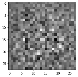
- The above image is that the generator has just tried to print without any train.
- It is just noise. Generator will gradually generates MNIST-like data while going through train ?
-
If you need more information about Batch Normalization, please, refer to the below article.
2.2. Discriminator
- Discriminator is an image classifier based on CNN.
def make_discriminator_model():
    model = tf.keras.Sequential()
    model.add(layers.Conv2D(64, (5, 5), strides=(2, 2), padding='same',
                                     input_shape=[28, 28, 1]))
    model.add(layers.LeakyReLU())
    model.add(layers.Dropout(0.3))

    model.add(layers.Conv2D(128, (5, 5), strides=(2, 2), padding='same'))
    model.add(layers.LeakyReLU())
    model.add(layers.Dropout(0.3))

    model.add(layers.Flatten())
    model.add(layers.Dense(1))

    return model
discriminator = make_discriminator_model()
decision = discriminator(generated_image)
print (decision)
tf.Tensor([[0.00050776]], shape=(1, 1), dtype=float32)
- This is important that this Discriminator is an image classifier, but it would not determine what the image generated by the generator is 0 to 9, but it is to determine whether the image generated by ** generator is fake or not. **
- So the output is dense(1).
- If it is judged to be real, it outputs a positive number, in case of fake, it outputs negative.
3. Loss Function & Optimizer
- Let’s make a loss function for G & D.
# This method returns a helper function to calculate Cross Entropy Loss (cross entropy loss).
cross_entropy = tf.keras.losses.BinaryCrossentropy(from_logits=True)
- BinaryCrossEntry gets two parameters, the first is the actual label, the second is the second is a prediction value.
3.1. Loss Function of Discriminator
- This method numerates how well the Discriminator determines the fake image and real image.
- Compare discriminator for real image and compare matrix made up of 1, and compare matrices that are predicted and 0 of discriminator for fake image.
def discriminator_loss(real_output, fake_output):
    real_loss = cross_entropy(tf.ones_like(real_output), real_output)
    fake_loss = cross_entropy(tf.zeros_like(fake_output), fake_output)
    total_loss = real_loss + fake_loss
    return total_loss
3.2. Loss Function of Generator
- The loss function of generator numerates how well generator deceives discriminator.
- If the generator is well trained, discriminator will classify fake image as real image (or 1).
- Here it will compare the decriminator’s decision on the generated image and compared with the matrix made up of one.
def generator_loss(fake_output):
    return cross_entropy(tf.ones_like(fake_output), fake_output)
- Because generator and discriminator are trained separately, we define optimizer separately.
generator_optimizer = tf.keras.optimizers.Adam(1e-4)
discriminator_optimizer = tf.keras.optimizers.Adam(1e-4)
3.3. Check Point
checkpoint_dir = './training_checkpoints'

checkpoint_prefix = os.path.join(checkpoint_dir, "ckpt")

checkpoint = tf.train.Checkpoint(generator_optimizer=generator_optimizer,
                                 discriminator_optimizer=discriminator_optimizer,
                                 generator=generator,
                                 discriminator=discriminator)
4. Define Train Loop
- Defining train loop.
- Defineing some contant values.
EPOCHS = 50
noise_dim = 100
num_examples_to_generate = 16

seed = tf.random.normal([num_examples_to_generate, noise_dim])
4.1. @tf.fuctnion Annotation
- @ tf.fuctNion allows you to compile a function and make it as Tensorflow 1.x Style.
- In Tensorflow 1.x, you first defined the network to use for train or inference. Thereafter, when using network, we opened a session to receive the input data to train, or use the network to do inference.
- It means that we always have to open a session to do some operation.
- One of the biggest changes as moving from Tensorflow 1.x to Tensorflow 2.x, the eager execution feature that can perform any calculations without a session concepts has been applied as default.
- We may have a question that most of them use Tensorflow 2.x, why it is left the annotation that can be used to write a method of 1.x yet, the reason is because of the speed.
- On Tensorflow 2.x, if you attach @ tf.fuctnion, you create a function as if you are creating and executing network as if Tensorflow 1.x.
- This allows you to benefit slightly depending on the situation, but debugging can be difficult.
- It is recommended that you attach @ tf.fuctnion when you think all the functions are confirmed.
4.2. Custom Train Loop
- Usually Tensorflow & Keras allows you to easily implement a model and test using various networks and functions that are already implemented.
- If you are prepared for data and definition of the loss function, optimizer definition, call .compile () / .fit (), the framework would do the forward propagation / back propagation, and weigh update.
- However, in certain cases, you may want to use model that is not yet supported by Tensorflow / Keras, or you want to control the train a little more closely.
- In this case, you can use the custom training feature in Tensorflow
- This DCGAN example also uses custom train loop.
4.3. tf.GradientTape()
- Network made using Keras / Tensorflow is very convenient because automatic differentiation will automatically calculate and do backprpgation.
- However, if you are using custom train loop as in this example, you must directly differentiation by yourself.
- Not all of them, but if you store the gradient when forwarding, you can save the differentiation much faster when you save the gradient.
- TF.GradientTape () is the role that stores the values that are required when forwarding the forward procagation.
- Keep the annotation mentioned above and let’s look at the train step function below.
@tf.function
def train_step(images):
    noise = tf.random.normal([BATCH_SIZE, noise_dim])

    with tf.GradientTape() as gen_tape, tf.GradientTape() as disc_tape:
        generated_images = generator(noise, training=True)

        real_output = discriminator(images, training=True)
        fake_output = discriminator(generated_images, training=True)

        gen_loss = generator_loss(fake_output)
        disc_loss = discriminator_loss(real_output, fake_output)

    gradients_of_generator = gen_tape.gradient(gen_loss, generator.trainable_variables)
    gradients_of_discriminator = disc_tape.gradient(disc_loss, discriminator.trainable_variables)

    generator_optimizer.apply_gradients(zip(gradients_of_generator, generator.trainable_variables))
    discriminator_optimizer.apply_gradients(zip(gradients_of_discriminator, discriminator.trainable_variables))
- After saving variables in tape during forward propagation, you can later know using variables that you saved prior to backPropagation.
- This is the actual train function.
- Since it’s a custom train loop, epoch control should be done by yourself.
def train(dataset, epochs):

    for epoch in range(epochs):
        start = time.time()

        for image_batch in dataset:
            train_step(image_batch)

        display.clear_output(wait=True)
        generate_and_save_images(generator,
                                 epoch + 1,
                                 seed)

        if (epoch + 1) % 15 == 0:
            checkpoint.save(file_prefix = checkpoint_prefix)

        print ('Time for epoch {} is {} sec'.format(epoch + 1, time.time()-start))

    display.clear_output(wait=True)

    generate_and_save_images(generator,
                           epochs,
                           seed)
def generate_and_save_images(model, epoch, test_input):
    predictions = model(test_input, training=False)

    fig = plt.figure(figsize=(4,4))

    for i in range(predictions.shape[0]):
        plt.subplot(4, 4, i+1)
        plt.imshow(predictions[i, :, :, 0] * 127.5 + 127.5, cmap='gray')
        plt.axis('off')

    plt.savefig('image_at_epoch_{:04d}.png'.format(epoch))
    plt.show()
5. Training
- The train() method defined above trains Generator and Discriminator at the same time.
- GANs, including DCGANs, can be very difficult to train.
- Because it is difficult to train the generator and discriminator at the same time in a balanced way
- As expected, the generated image is not quite clear at the beginning, but as the epoch progresses, it looks more and more like a number.
%%time
train(train_dataset, EPOCHS)

Wall time: 20min 44s
6. Make GIF
- In order to see the train process more visually, let’s make it into an animation GIF.
- Let’s load the model from our last checkpoint.
checkpoint.restore(tf.train.latest_checkpoint(checkpoint_dir))
<tensorflow.python.training.tracking.util.CheckpointLoadStatus at 0x26c587ad3a0>
def display_image(epoch_no):
    return PIL.Image.open('image_at_epoch_{:04d}.png'.format(epoch_no))
display_image(EPOCHS)

anim_file = 'dcgan.gif'

with imageio.get_writer(anim_file, mode='I') as writer:
    filenames = glob.glob('image*.png')
    filenames = sorted(filenames)
    last = -1

    for i,filename in enumerate(filenames):
        frame = 2*(i**0.5)

        if round(frame) > round(last):
            last = frame
        else:
            continue

        image = imageio.imread(filename)
        writer.append_data(image)

    image = imageio.imread(filename)
    writer.append_data(image)

import IPython

if IPython.version_info > (6,2,0,''):
    display.Image(filename=anim_file)
- As you look in the folder, you can see that the ‘dcgan.gif’ file is created.
- Looking at this file, you can see how the train process went.