Batch Normalization (EN)
Batch Normalization
0. Introduction
0.1. Gradient Vanishing / Exploding
- It tunes parameters by examining changes in gradient values during neural network training.
- Gradient(derivative) is the amount of change. As the depth of the neural network depp, the gradient values do not properly reflect the change in the input value of the input layer during backpropagation in training.
- During backpropagation, if you use non-linear activation functions (Ex. Sigmoid / Tanh ), the gradient values become smaller (Gradient Vanishing) or conversely, the gradient values become larger (Gradient Exploding) as the layer passes through. A situation arises that the amount of change in the output layer cannot be properly reflected in the parameters of the neural network.
- Several methods have been proposed to improve this problem.
0.2. Countermeasure of Gradient Vanishing / Exploding
-
Applying ReLU
Since the root cause is the use of the non linear activation function, this is the method of using the linear activation function like ReLU.
-
Special Weight Initialization
It is known that this problem can be improved by properly initializing the layer’s weight value. He initialization or Xavier initialization are well-known weight initialization methods.
- Applying Small Learning Rate
0.3. Fundamental Solution
- The methods mentioned above are all indirect ways to improve Gradient Vanishing / Exploding.
- Batch Normalization came out of researching a fundamental solution.
1. Batch Normalization
- The paper introducing Batch Normalization is titled ‘Batch Normalization: Accelerating Deep Network Training by Reducing Internal Covariate Shift’.
-
Please, refer to the below link of paper
1.1. Advantage of Batch Normalization
Known Batch Normalization benefits are :
-
Training speed gets faster.
It might be the most important advantage. The performance is the same or better than that of not applying batch normalization, but converges quickly with fewer epochs. Some says it’s at least 10 times faster.
-
The sensitivity of the network to hyper parameter is reduced.
Generally, we tune hyper parameter when the performance wasn’t good. It can greatly reduce the burden on it.
-
There is a regularization effect.
Better performance during inference.
1.2. Adding Batch Normalization Layer
- Add Batch Normalization layer in the middle of the hidden layer as shown in the figure below.
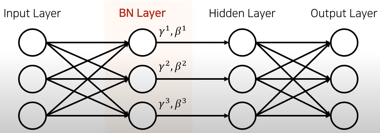
- More specifically, it is said that putting it in front of the activation function gives better results experimentally.
- The key to batch normalization is to properly control the output value of the previous layer before passing it on to the next layer by adding two parameters γ and β as many as the number of output neurons in the previous layer.
- There is no reason not to apply batch normalization because the performance of the network increases dramatically by adding only the cost of calculating two parameters.
2. Background
2.1. Normalization
- The normalization technique that makes each feature have a similar range of values is used in many fields, and it improves the training speed.
- The reason why the training speed increases when applying normalization is that it is difficult to use a large learning rate if the variation for each feature is different, so the training speed cannot be increased quickly.
2.2. Standardization
- A method similar to normalization is standardization.
- This is a method to make the distribution of features a mean of 0 and a variance of 1.
3. Implementation of Batch Normalization
- It is simple to put a normalized feature in the first input layer. It can be normailzed while pre-processing and input into network.
- However, if the input data distribution of the hidden layer is different every time and it is not normalized, the network would not be trained well.
- Then, how would it be if the input data is normalized each hidden layer ? The simplest and most ignorant way is to normalize it before passing it on to each hidden layer.
3.1. Batch Normalization
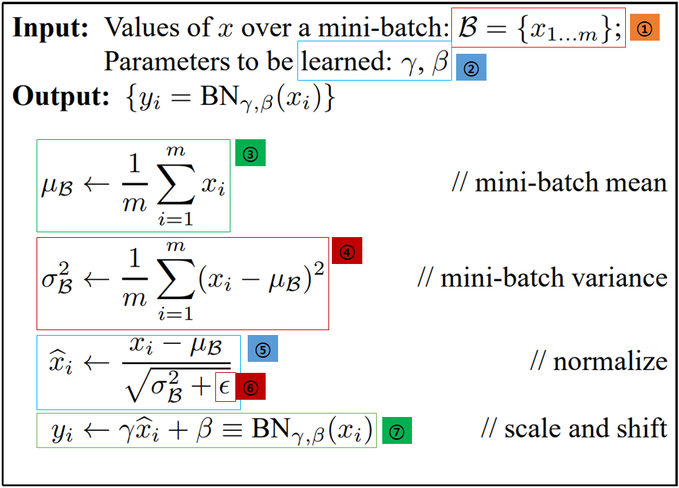
- The formula below is the calculation method of the input and output values of batch normalization shown in the paper.
-
1 : First, let’s look at the values that are input to batch normalization.
In mini-batch, it comes in as input as x1 ~ xm. Here, you can think of m as the batch size. More specifically, it will be the activation output value of the previous layer.
- 2 : These two values of γ and β are the values we actually need to train. With these values, you control the values that will go into the next layer. Two γ and β for each input value.
- 3 : Calculating the average value of mini-batch.
- 4 : Calculating the variance of mini-batch.
- 5 : Normalizing.
- 6 : Adding a very small value to prevent division by zero.
- 7 : Finally, it is the output value that has been applied to batch normalization.
- γ,(Scale) and β(Bias) will be changed through the process of learning in the direction in which the neural network performance improves (the direction in which loss decreases).
4. Effect of Batch Normalization
- The benefits achieved with Batch Normalization are undisputed.
- As mentioned earlier, the train speed is fast and frees you from hyper parameter tuning.
- As checking the train results under various conditions, you can see that the train speed is definitely fast when batch normalization is applied and converges quickly even with a large learning rate.

5. Algorithm of Training & Inference
- Let’s check how to apply batch normalization in train / inference steps introduced in Paper.
- The difference from other networks when applying batch normalization is that the networks for train and inference are different.
- Another reason is that the mean and variance of the data used for training are different from the mean and variance of the data used during inference.
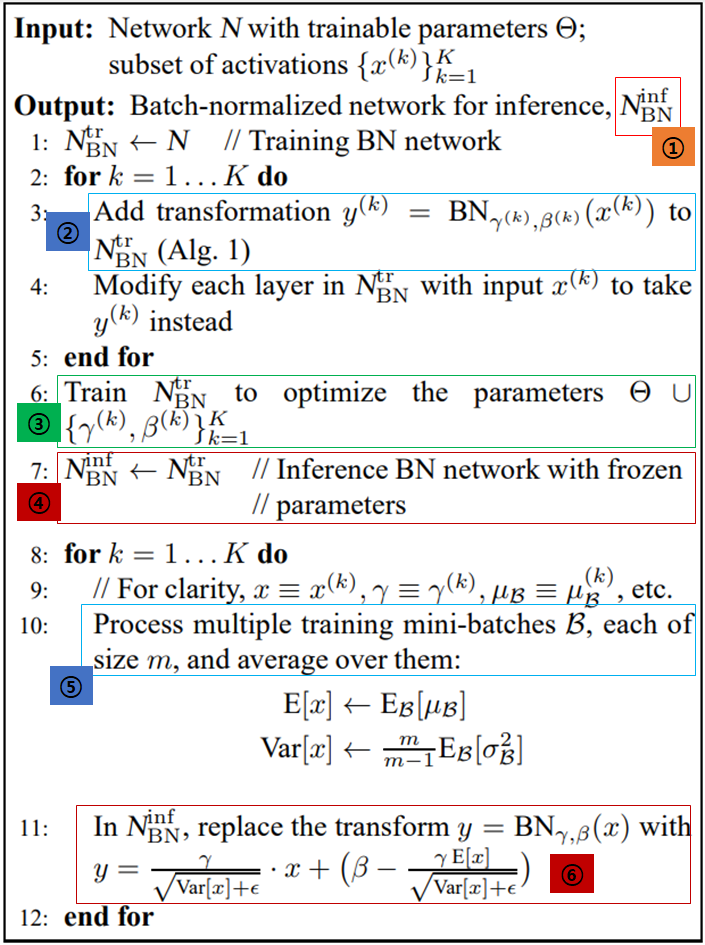
- 1 : The final purpose of this algorithm is to obtain a network for inference with batch normalization applied.
- 2 : It means adding a batch normalization layer to the existing network.
- 3 : Training γ and β with batch normalization layer added.
- 4 : After training, fixing the parameters and change the network to inference mode.
- 5 : Calculate mean and variance using several mini batch with train data.
- 6 : In inference, a moving mean is used.
6. Essence of Batch Normalization
- In this time, we’ll see why batch normalization works so well.
6.1. Covariate Shift
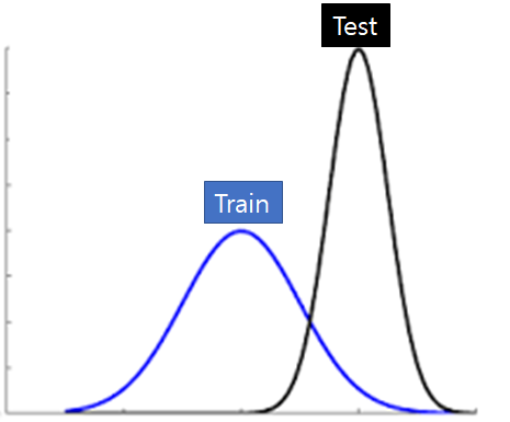
- Covariate shift refers to a phenomenon in which the data distribution used for training and the data distribution used for testing change.
6.2. Internal Covariate Shift ( ICS )
- ICS(Internal Covariate Shift) means a phenomenon in which covariate shift occurs inside the network and this is the problem that batch normalization tried to solve.
- It means that the input data distribution is different each time in the back layer and the deeper the layer, the more serious it gets.
- After the publication of batch normalization, it was known that the performance improvement factor of batch normalization was not related to the reduction of ICS.
-
Paper - How Does Batch Normalization Help Optimization?
6.3. Batch Normalization & Internal Covariate Shift ( ICS )
- Even if ICS is forcibly generated by inserting random noise right after batch normalization layer, it still shows good performance.

6.4. Smoothing Effect of Batch Normalization
- Batch Normalization has the effect of smoothing the optimization landscape.
- Optimization landscape is a visualization of the change in loss according to weight.
- The picture below is optimization landscape. The left side shows no batch normalization and the left side shows batch normalization.
- As you can see, in the case of the left optimization landscape, you can see that the loss is very jagged in weight domain.
- On the other hand, in the case of optimization landscape on the right, it can be seen that the loss value distribution is very smooth.
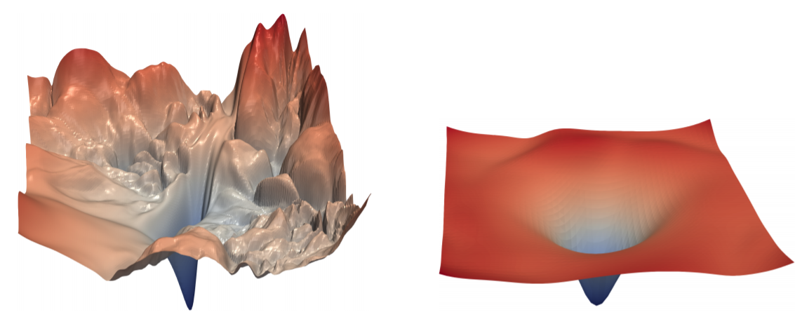
- It is known that it has not only batch normalization, but also residual connection that has smoothing effect.
- Predictiveness is a measure of how reliable the current gradient direction is.
- In the first picture, when batch normalization is applied, the change in loss itself is small and the change in loss is not large even if it moves a lot.
- Similarly in the second picture, moving the slope with a large step does not change much.
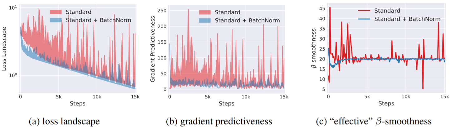
- In summary, if batch normalization is applied, the gradient after moving is highly likely to be similar to the present even if a large step is moved in the direction of the current gradient.